Synthesize signals from lifetimes

An introduction to the lifetime_to_signal function.

The phasorpy.lifetime.lifetime_to_signal() function is used to synthesize time- and frequency-domain signals as a function of fundamental frequency, single or multiple lifetime components, lifetime fractions, mean and background intensity, and instrument response function (IRF) peak location and width.

Import required modules and functions:

import numpy
from matplotlib import pyplot

from phasorpy.lifetime import (
    lifetime_to_signal,
    phasor_calibrate,
    phasor_from_lifetime,
)
from phasorpy.phasor import phasor_from_signal

Define common parameters used throughout the tutorial:

frequency = 80.0  # fundamental frequency in MHz
reference_lifetime = 4.2  # lifetime of reference signal in ns

lifetimes = [0.5, 1.0, 2.0, 4.0]  # lifetimes in ns
fractions = [0.25, 0.25, 0.25, 0.25]  # fractional intensities

settings = {
    'samples': 256,  # number of samples to synthesize
    'mean': 1.0,  # average intensity
    'background': 0.0,  # no signal from background
    'zero_phase': None,  # automatic location of IRF peak in the phase
    'zero_stdev': None,  # standard deviation of time-domain IRF in radians
}

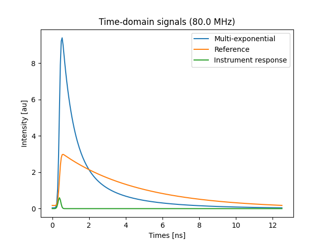
Time domain, multi exponential

Synthesize a time-domain signal of a multi-component lifetime system with given fractional intensities, convolved with an instrument response function:

signal, instrument_response, times = lifetime_to_signal(
    frequency, lifetimes, fractions, **settings
)

A reference signal of known lifetime is required to calibrate the phasor coordinates. The reference signal must be obtained with the same instrument and sampling parameters. The calibrated phasor coordinates match the theoretical phasor coordinates expected for the lifetimes:

reference_signal, _, _ = lifetime_to_signal(
    frequency, reference_lifetime, **settings
)


def verify_signal(reference_signal, fractions=None):
    """Verify calibrated phasor coordinates match expected results."""
    assert numpy.allclose(
        phasor_calibrate(
            *phasor_from_signal(signal)[1:],
            *phasor_from_signal(reference_signal),
            frequency,
            reference_lifetime,
        ),
        phasor_from_lifetime(frequency, lifetimes, fractions),
        atol=1e-3,
        equal_nan=True,
    )


verify_signal(reference_signal, fractions)

Plot the synthesized signals (multi-exponential, reference, and instrument response):

fig, ax = pyplot.subplots()
ax.set(
    title=f'Time-domain signals ({frequency} MHz)',
    xlabel='Times [ns]',
    ylabel='Intensity [au]',
)
ax.plot(
    times,
    # scale IRF peak to match signal peak
    instrument_response * (signal.max() / instrument_response.max()),
    linewidth=0.8,
    color='tab:grey',
    label='Instrument response',
)
ax.plot(times, signal, label='Multi-exponential')
ax.plot(times, reference_signal, label='Reference')
ax.legend()
pyplot.show()

Time domain, single exponential

To synthesize separate signals for each lifetime component at once, omit the lifetime fractions:

signal, _, times = lifetime_to_signal(frequency, lifetimes, **settings)

verify_signal(reference_signal)

Plot the synthesized signals:

fig, ax = pyplot.subplots()
ax.set(
    title=f'Time-domain signals ({frequency} MHz)',
    xlabel='Times [ns]',
    ylabel='Intensity [au]',
)
ax.plot(times, signal.T, label=[f'{t} ns' for t in lifetimes])
ax.legend()
pyplot.show()

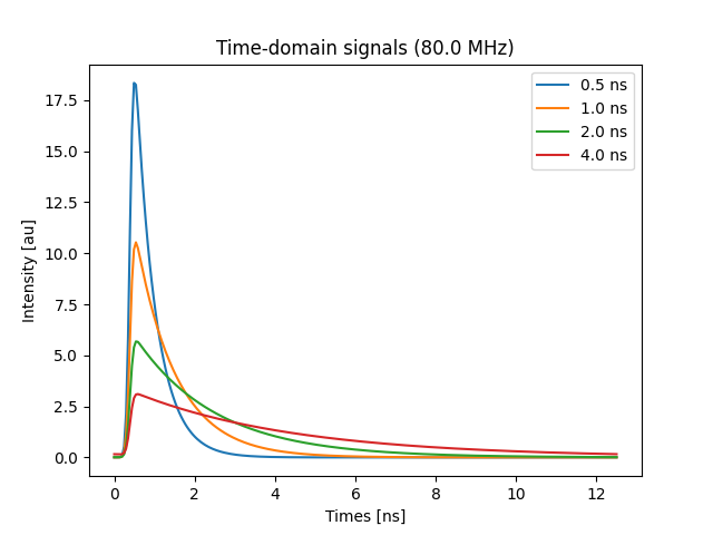
As expected, the shorter the lifetime, the faster the decay.

Frequency domain, multi exponential

To synthesize a frequency-domain homodyne signal, limit the synthesis to the fundamental frequency (harmonic=1):

signal, instrument_response, _ = lifetime_to_signal(
    frequency, lifetimes, fractions, harmonic=1, **settings
)

reference_signal, _, _ = lifetime_to_signal(
    frequency, reference_lifetime, harmonic=1, **settings
)

verify_signal(reference_signal, fractions)

Plot the synthesized signals:

phase = numpy.linspace(0.0, 360.0, signal.size)

fig, ax = pyplot.subplots()
ax.set(
    title=f'Frequency-domain signals ({frequency} MHz)',
    xlabel='Phase [°]',
    ylabel='Intensity [au]',
    xticks=[0, 90, 180, 270, 360],
)
ax.plot(
    phase,
    instrument_response,
    linewidth=0.8,
    color='tab:grey',
    label='Instrument response',
)
ax.plot(phase, signal, label='Multi-exponential')
ax.plot(phase, reference_signal, label='Reference')
ax.legend()
pyplot.show()

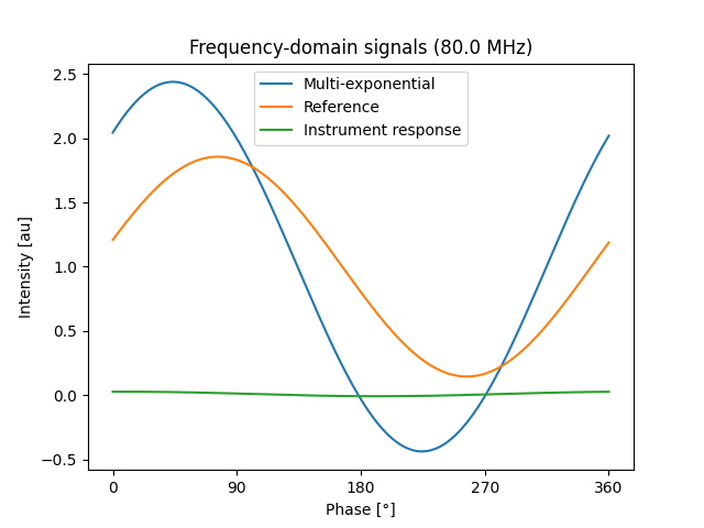
The homodyne signal can contain negative values since the modulation depth of the excitation source is 1.

Frequency domain, single exponential

To synthesize separate signals for each lifetime component at once, omit the lifetime fractions. Halving the modulation depth of the excitation source (zero_modulation=0.5) guarantees a non-negative signal for any lifetime:

signal, _, _ = lifetime_to_signal(
    frequency, lifetimes, harmonic=1, zero_modulation=0.5, **settings
)

reference_signal, _, _ = lifetime_to_signal(
    frequency, reference_lifetime, harmonic=1, zero_modulation=0.5, **settings
)

verify_signal(reference_signal)

Plot the synthesized signals:

fig, ax = pyplot.subplots()
ax.set(
    title=f'Frequency-domain signals ({frequency} MHz)',
    xlabel='Phase [°]',
    ylabel='Intensity [au]',
    xticks=[0, 90, 180, 270, 360],
)
ax.plot(phase, signal.T, label=[f'{t} ns' for t in lifetimes])
ax.legend()
pyplot.show()

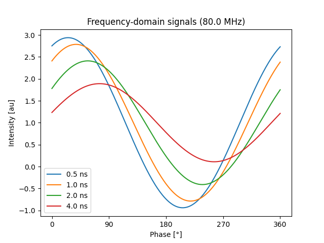
As expected, the shorter the lifetime, the smaller the phase shift and demodulation.