Interactive applications

Explore phasor concepts using interactive educational applications.

The PhasorPy library includes interactive applications for educational purposes. They open graphical user interfaces where parameters can be adjusted via sliders and the resulting phasor, lifetime, and spectral plots are updated in real time. The applications can be started from the Command-line interface or programmatically. A matplotlib backend that supports interactive windows is required.

Lifetime application

Interactively plot time-domain signals, phasor coordinates, and multi-frequency phase and modulation curves for a set of lifetime components and their mixture at given frequency and fractional intensities.

Start the lifetime app with three components from the command line:

$ python -m phasorpy lifetime 3

or run the following code in a Python interpreter:

from phasorpy.plot import LifetimePlots

LifetimePlots(
    frequency=80.0,  # MHz
    lifetime=(0.4, 3.4, 8),  # ns
    fraction=(0.3, 0.5, 0.2),  # fractional intensities
    interactive=True,
).show()

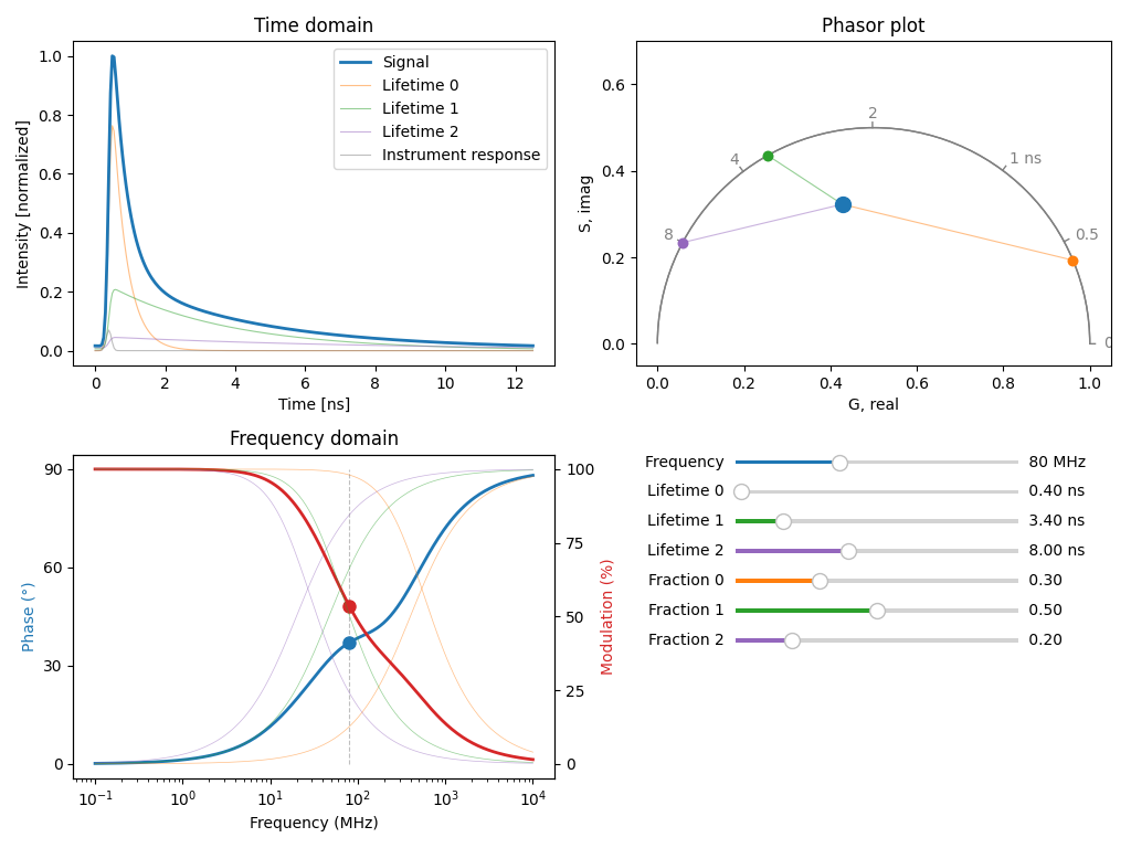
Change frequency, lifetimes, and fractional intensities to see how the phasor coordinates, phase and modulation, and decay curves respond.

Spectral application

Interactively plot emission spectra and spectral phasor coordinates for one or more spectral components and their mixture over a selectable wavelength range.

By default, each component is modelled as a Gaussian in wavelength space. Shifting the origin rotates the phasor without changing the modulation (provided the spectrum fits within the wavelength window), and changing sigma alters the modulation independently. Optionally, the Displaced Harmonic Oscillator (DHO) model can be used for more realistic fluorophore spectra with vibronic structure (dho=True).

Start the spectral app with two components from the command line:

$ python -m phasorpy spectral 2

or run the following code in a Python interpreter:

from phasorpy.plot import SpectralPlots

SpectralPlots(
    origin=(500.0, 580.0),  # center wavelengths in nm
    sigma=(20.0, 40.0),  # Gaussian widths (standard deviations) in nm
    fraction=(0.6, 0.4),  # fractional intensities
    wavelength_range=(400.0, 700.0),
    interactive=True,
).show()

Change the wavelength range, number of samples, origin, and sigma sliders to see how the spectrum shape and phasor position respond. Narrow the wavelength window until a Gaussian is truncated to observe how clipping the spectrum reduces the modulation.

FRET application

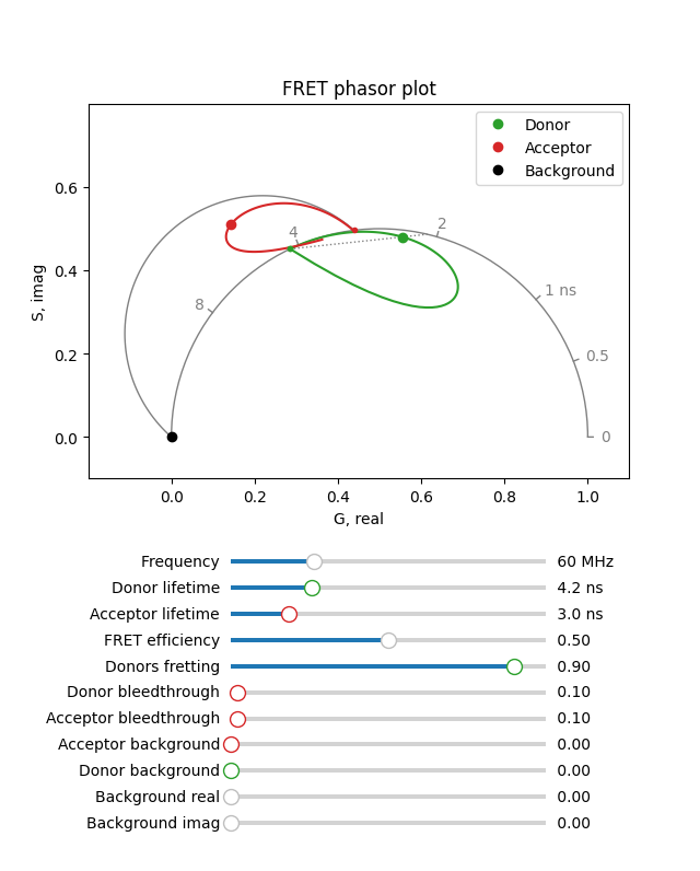
Interactively plot phasor coordinates for Förster resonance energy transfer (FRET) donor and acceptor channels as a function of frequency, donor and acceptor lifetimes, FRET efficiency, fractions of donors undergoing FRET (donor fretting), donor and acceptor bleedthrough, and background signal.

Start the FRET app from the command line:

$ python -m phasorpy fret

or run the following code in a Python interpreter:

from phasorpy.plot import PhasorPlotFret

PhasorPlotFret(
    frequency=60.0,  # MHz
    donor_lifetime=4.2,  # ns
    acceptor_lifetime=3.0,  # ns
    fret_efficiency=0.5,  # 50%
    donor_fretting=0.9,  # 90% of donors can undergo FRET
    donor_bleedthrough=0.1,  # 10% donor signal in acceptor channel
    acceptor_bleedthrough=0.1,  # 10% acceptor signal in donor channel
    interactive=True,
).show()

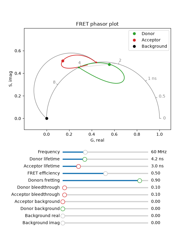
Change frequency, FRET efficiency, lifetimes, and bleedthrough fractions to see how the donor and acceptor phasor positions respond.